Week 5: Machine Learning Ramps Up
Monday July 22, 2019
Hi everyone! I can’t believe we’re already nearing the end of July! Is it just me or is this summer seriously flying by?? Anyways, today was major progress on the third part of my project: classification using machine learning! So just a quick recap, there’s an article by the Smithsonian explaining how they were able to use a ML algorithm to sort two plant families that are morphologically similar (Lycopodiaceae and Selaginellaceae). Check it out here! They also used an algorithm to find stained specimen sheets, but for now, we’re only focused on the family part. My current goal is to understand machine learning enough to essentially replicate what they did in the article. Then after that, we would like to apply a similar concepts to other species or categories. For example, with the staining example done in the article, there’s a really practical purpose to conduct that. Essentially, in the past, specimen were treated with mercury to preserve them longer, but over time, we’ve learned that this is actually bad for the specimen and it causes staining on the specimen sheets. Eventually, we’d like to find the specimen that have been treated and are now stained so we can remount them, allowing them to last longer.
Last week, I created scripts to do a lot of the initial image processing so all the pictures are the same size (256 pixels by 256 pixels) and have the same resolution (96 ppi). Today, I started creating my own ML model using tensorflow and keras to train a model, following the tutorial here (bless the people who make easy to follow tutorials like this one!) Before I started attempting to recreate the model from the Smithsonian paper, I just wanted to get something working with the model in the tutorial and I did! I only used 100 images from each family and 10 epochs (epoch = essentially a cycle) and the accuracy is pretty trash, as you can see below.

Now that I have that, I plan to follow these steps:
- Change the layers to recreate the model from the Smithsonian Paper
- Increase my training size
- Test the model on a test batch!
Starting on step 1, I was almost able to finish replicating the paper’s model in Python. Although the Smithsonian used Mathematica, with the help of Google (honestly, I don’t know what I’d do on this project without Google) I think I’m able to figure out what the paper’s layers are doing then finding the relative equivalent in Python. I’ve almost finished that and hope tomorrow I’ll be able to get a small batch tested with hopefully higher accuracy than the random one I used today. Something I would like to investigate further is how do we know how many layers or filters to use? What filter size should we use for the convolution layer? How did they figure out what combination of layers worked best? It seems that creating a model is not that difficult, it’s the why you choose certain characteristics of the model that I’d like to further explore.
Well today was a very satisfying day and tomorrow we have our Python workshop! Can’t wait :D
-Al
Tuesday July 23, 2019
Hello! First thing I would like to talk about today is that I co-hosted my first Python workshop! It was for the other interns in the botany department as well as paleobotany and some high school interns. I think as a self reflection, overall it went pretty well! I think there was just a lot of information at once, especially for people who never used Python before. So in the future, if I were to do it again, I would be more careful about tailoring the workshop to the audience because of course everyone is at a different stage of learning! I sent out a feedback form, so hopefully that will help me become a better teacher in the future!
More related to my project, I think I got a model that’s pretty similar to the one described in the Smithsonian paper. At least by what the layers are called/what I think they do. The difficult part in this was because the paper was done in Mathematica while I’m using TensorFlow in Python, so the types of layers/how to use them don’t carry over exactly. I’ve been doing a lot of research into what certain layers are intended to do in Mathematica and trying to find the Keras/TensorFlow equivalent for Python.
With my first test, I used 100 images from each family (Lycopodiaceae and Selaginellaceae) to train/validate the model (10% of this batch are used for validation). The results of the accuracy are below:
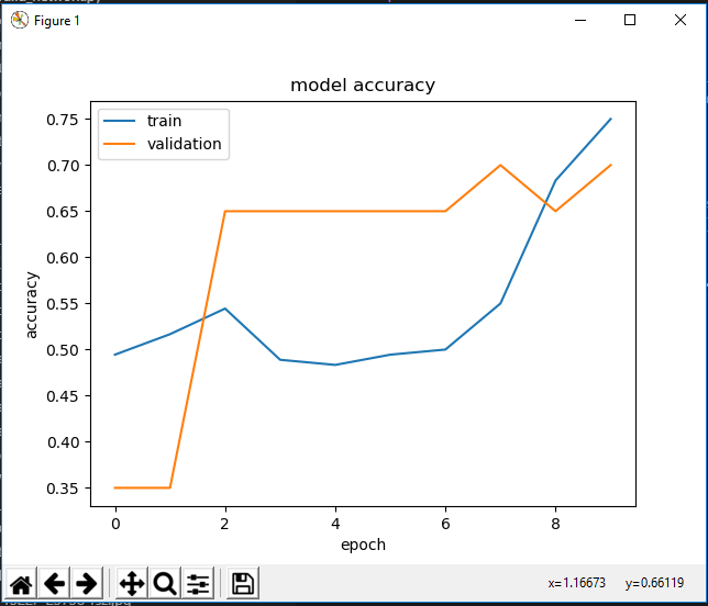
Although the training accuracy increased over time, we see that by the second epoch, the validation accuracy plateaued, which is not a good sign. Additionally, when tested on the same test data as above, all the images were labeled as Selaginellaceae, leading me to believe overfitting is happening, but I can look into this more tomorrow.
Exciting things are happening and I’m definitely kept busy!
-Al
Wednesday July 24, 2019
Today I took a bit of a break from the machine learning classification project. In the morning, a teacher from Northside College Prep came in and worked with us to create our own ozone detection strips! These strips can be used as indicators to see whether there are high levels of ozone in our area or not! They’re actually really easy to make; it was essentially mixing some cornstarch and water, add some sodium iodide, and painting them onto strips. Then we have to let them sit overnight.
The majority of the afternoon was spent helping out some scientists and the high school Digital Learning Interns, but I did get to work on the CNN model a little bit. To combat the issues I faced yesterday, I decreased the learning rate of the model from the standard for Adam (0.001) to 0.0001 and that improved our accuracy for training and validation (see below).
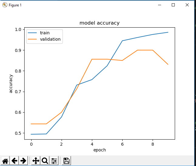
It looks nice, but I believe the model is still overfitting to the training data. This hypothesis was supported when I tested the model on some test data with 10 images from each family and all of them were labeled as Lycopodiaceae (the opposite from last time). Online says this may be due to imbalance of input data in training, but I don’t think that’s the case because we have 800 of each family. Maybe not enough data? I still believe overfitting is an issue here, so we need to see how we can reduce that. It may be time to consult some experts.
Although they’re tough, roadblocks are good! This means we’re learning :)
-Al
Thursday July 25, 2019
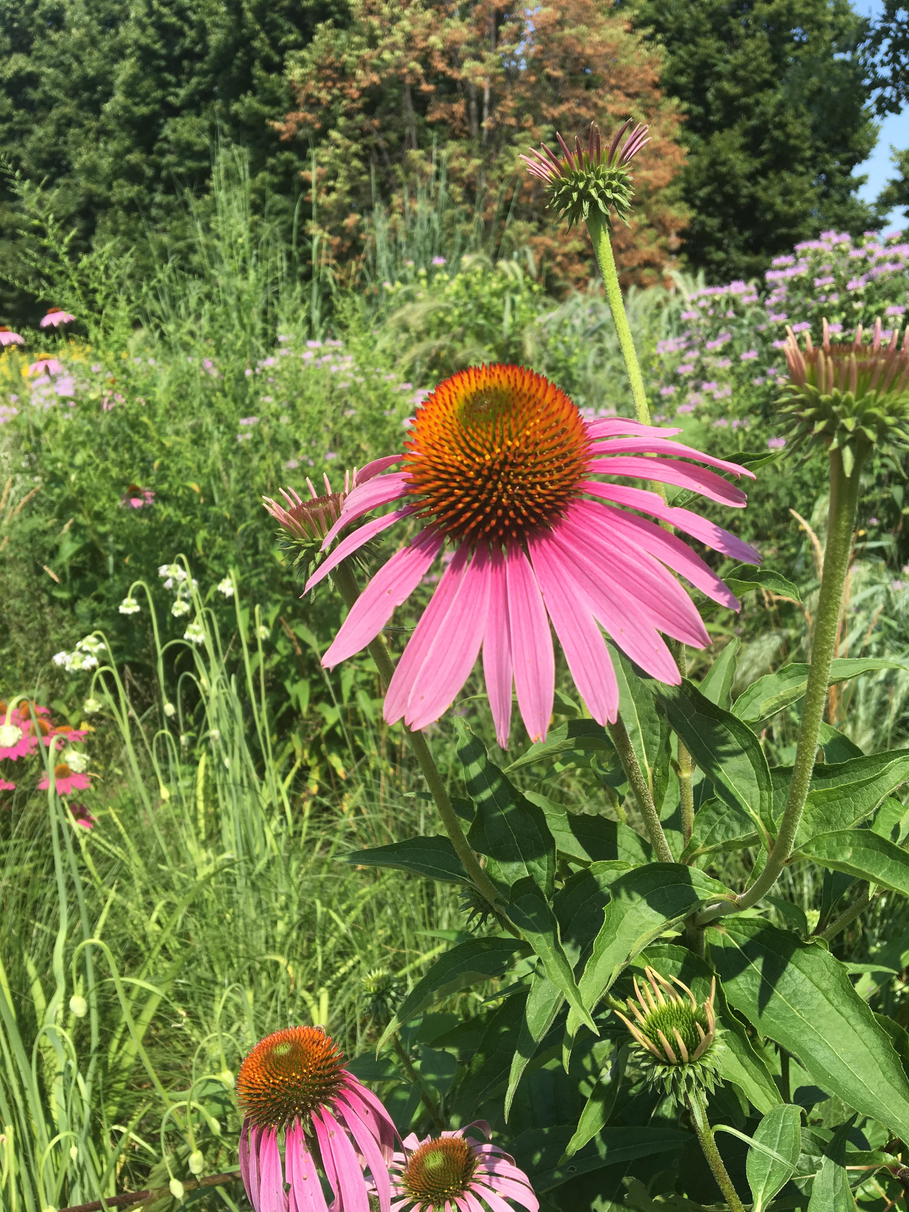
Happy Thursday! In the morning, we did a bit work with the ozone strips we prepped yesterday. We took them outside for a bit and tomorrow morning we can scan them to see the ozone levels found. It was nice to just walk outside around the museum and appreciate the gardens and all, like this nice picture below!
With the machine learning project, I noticed that overfitting was still occurring with our training model. Looking online, I found that Regularization could help. I did see L2 Regularization in the Smithsonian paper, but didn’t quite understand what was happening and didn’t implement it yet. The Smithsonian paper set the L2 Regularization to 5 which I found very odd because doing some research online, it seemed that regularization values were generally very small, less than 1. Additionally, in Mathematica, L2 Regularization is something set for the model as a whole, but in Keras, it’s done layer by layer. Keras also gives options for regularization in bias, activity, and kernel, so for now, I just created a new layer after the first Dense layer and set all the regularizers to 0.01.
There is no better way to describe my experience right now than research, guess, and check.
Additionally, I found you can add custom functions which would help match my dropout layer to the Smithsonian one. I found that the Mathematica dropout layer not only drops half the values, but also multiplies the remaining ones by 2, but dropout in Keras only drops a certain percent of the values. Creating a custom function, I used the basis of the relu activation function with two changes:
- I made the slope for negative values still 1, essentially making it an identity function
- I multiplied the function by 2
The model is running and saves, but when we want to load the model to test it, it’s unable to recognize my custom function which is something I’m still trying to figure out. In the end, I eventually took out the custom part because at this point, I’m not even able to test the model. Also, at the end of the day, I was training the model, but unfortunately left in a rush to catch my train. I’m not sure if this is normal, but I noticed that training the model takes up a LARGE majority of the computer’s memory and CPU, so that’s something I plan to look into tomorrow. I think before I continue tweaking and testing, it will be a good idea to update everyone from NEIU with what I’ve done (which may end up being completely useless) and just trying to learn more instead of just trying random things I find because that method is proving to be expensive (in matters of time)
Stay tuned!
-Al
Friday July 26, 2019
First, I’d just like to say we need to make more of an effort as a community to create a better world. To use less resources, less energy, and think every day how wecan make a positive environmental impact on this world. It’s all about give and take, not just always taking. I for one am going to look into making even just small daily habit changes that can add up to make a much larger impact. Anyways, regarding my machine learning project, today I made a break through! I was struggling for the last few days because although the training and validation accuracies would be okay, when it came to the testing data, basically the model just associated one class with all the data, even when I shuffled the data before testing. Well, after spending hours and hours researching, today I finally realized why, and it’s actually quite a dumb reason, so drumroll please!
…
…
…
It’s because I didn’t scale the RGB values of the pixels in the testing data!!! Basically, for the training model, we scaled all the RGB values for each pixel (usually between 0 and 255) to be between 0 and 1, but I forgot to do the same for the training data! So of course we wouldn’t be getting correct predictions!
After making that change, things began working again and I was actually able to make predictions! Initially, without making changes to the initial model, I was able to get about 93% accuracy with my test data, and now I’m working on changing my model to have it more closely match the Smithsonian paper and seeing the effects. I started to see a little overfitting, so I’ve been increasing drop out and decreasing learning rate, for example, to combat that. I’ve also been keeping a record of my changes and results. Check it out for an always up to date record!
I won’t be in at all next week because I’m going to Pittsburgh, but this has been a great place to stop for myself!
-Al